
Working with studio headphones and monitors that feature the flattest frequency responses is important. They reduce the possible variation our listener's will hear due to their own stereo systems, equalization preferences, and the influence of their listening rooms.
Untold hours and billions of dollars have been spent in research and development in these industries alone.
Then two physicists stepped into the game and changed everything.
Fletcher and Munson disrupted the recording industry and home stereo and entertainment system industries in such a way that we still talk about the impact and implications 84 years later.
The groundwork they laid in 1933 led to further investigation on the topic and to eventual international standards used in the manufacturing and research of audio-related products and studies.
Let's jump in and get a quick history on the development of these perceived loudness curves and then take a look at how it should impact our mixing and mastering workflow to help us produce higher quality results for our artists and fans.
First, let's define what this curve is and represents, then dig into the history of this insightful discovery:
What is the Fletcher Munson Curve?
The Fletcher Munson Curve is the first of several measurements that came to be called equal-loudness contours. These contours are visual diagrams displaying the effect that loudness and frequency has on human hearing.
With all of the focus on the frequency response of diaphragms and mechanisms that reproduce sound, such as speakers and acoustic environments, nobody considered the biological organs that perceive sound.
The aforenamed scientists considered the problem on a higher order and measured the influence the human ear has on perceiving volume, pitch, and the relative loudness level of each frequency range compared to one another. He then launched one of the earliest studies in psychoacoustics ever.
The History of Fletcher & Munson's Loudness Curves
It all began when lead researcher Harvey Fletcher and Wilden A. Munson published their seminal paper in the Journal of the Acoustic Society of America entitled "Loudness, its definition, measurement and calculation."
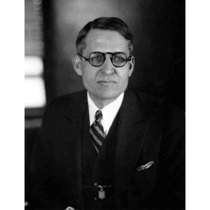
Harvey Fletcher, an American physicist born on September 11, 1884 and perished on July 23, 1981, had an illustrious career in acoustics, music, television, and many other scientific and engineering disciplines. Among his achievements:
- the invention of the 2-A audiometer
- creating one of the earliest hearing aids
- contributing to experiments that earned a Nobel Prize for Physics
- membership in countless scientific societies
- and the accolade of being known as the father of stereophonic sound.
In their paper, the acoustic research duo developed the concept of what came to be known as the equal-loudness contour, a grouping in which their original curve is but one sub-set. The two are commonly and incorrectly used as synonymous.
The purpose of the paper was to publish the methodology and results of measuring as accurately as possible the sensitivity of the human ear in relation to loudness and frequency.
Their conclusion and diagrams showed that human perception of frequency has an undoubtable dependence on the amplitude of each frequency.
The most important revelation from these findings is that human hearing is most sensitive to frequencies within the band between 3 kHz and 4 kHz.
The implication is that, depending on the average volume, all frequency ranges outside of the 3 kHz to 4 kHz range must be as much as 10 decibels louder to be perceived as being at the same volume.
The Fletcher Munson Diagram
Below is a large sized image of the Fletcher Munson diagram including all of the reported data.
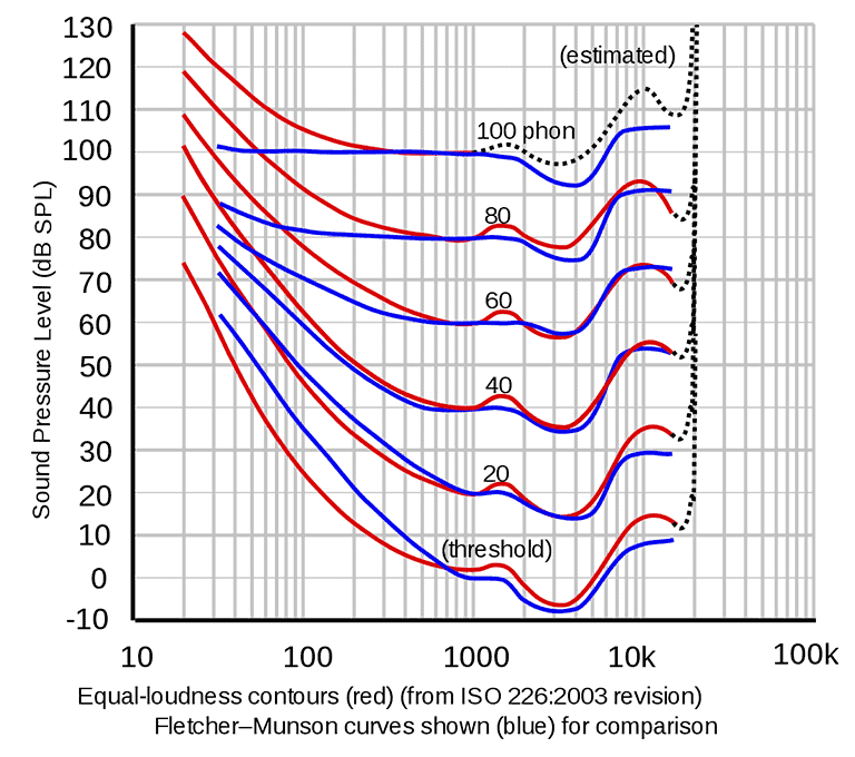
The blue lines are the data reported in the original research. The red lines follow the measurements by Robinson and Dadson, which we'll discuss next, that ultimately become the current equal loudness contour international standard.
Both are plotted logarithmically on the horizontal access across the frequency spectrum of human hearing. On the vertical access are sound pressure levels from -10 dB up to 130 dB, allowing us to see six sets of measurements at once at 20 dB increments.
The dip between 3 kHz and 4 kHz correlates to the increased sensitivity of the human ear in that range, as mentioned above. A slight increase of 2 dB to 5 dB occurs between 1 kHz and 2 kHz, while an even greater sensitivity appears linearly up between 4 kHz and 11 kHz.
This is an inverse relationship, which means these regions require less loudness for humans to perceive them as being the same volume as louder frequencies.
Note that while the two sets of curves are relatively similar above 500 Hz, they differ quite drastically in the bass and sub-bass regions.
It's accepted that the Robinson Dadson Curve is more accurate, although the original curve continued to relate more closely to all other standards all the way until the ISO 226 standard was adjusted in 2003.
The discrepancies in the bass and sub-bass frequency ranges have been attempted to be explained away, yet no explanation has been deemed satisfactory, by saying:
- The measuring devices weren't properly calibrated for those regions
- The judging criteria has changed over the years, varying for different frequencies
- The subjects were suffering from over-exposure to low-frequency sounds before testing
- The race of the participants had an effect (inclusion of Japanese data)
Any proper experiment that has been accepted as an international standard will have controlled for listener fatigue, so we can rule that out. It's important to note that sub-bass frequencies are felt more than heard, so that's partially why this discrepancy has been glossed over.
The Robinson Dadson Curve
The current ISO 226 standard is based on the Robinson Dadson curves as reported in the British Journal of Applied Physics in a paper entitiled "A re-determination of the equal-loudness relations for pure tones." D. W. Robinson and R. S. Dadson's work was surprising to say the least.
Various standards had been accepted in the time between the original report and that of Robinson and Dadson. The latter's published data varied more significantly from the time's current standard and average of other results than did any other.
Fortunately, the original 40-phon measurement, which was the basis for the A-weighting standard, agreed quite well with the Robinson Dadson 40-phon measurement (as seen above in the diagram), which brought confidence for the rest of the measurements.
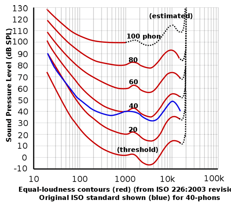
Above are the current standards, the ISO 226 standard based on Robinson and Dadson's reported data, but adjusted using recent assessments by researchers across the globe in 2003. The blue line is the original ISO standard for 40-phons, which is not to be confused with the original 40-phon curve.
The adjustments, to everyone's relief, brought the data back into reconciliation with the data from the initial paper, especially in the bass regions.
This is currently deemed the most accurate measurement and is used internationally by all professionals, despite the questionably fluctuating results in the bass and sub-bass frequency ranges.
Equal Loudness Contours: Methodology
We've focused on the results, but how does an equal loudness curve get measured? We can't rely on self-reporting by listeners because subjective data can't be objectively compared. So how is a human hearing curve built?
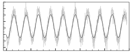
The basic methodology is the playing of two pure tones using sine waves at set frequencies and at incremented sound pressure levels (volumes) while having a listener report when they perceive the two as being at equal volumes.
The participants must be an average youth with no significant hearing loss. Any reported hearing impairment disqualifies a person from the experiment.
It has been determined that the human auditory system can perceive frequencies from around 20 Hz up to around 22 kHz. The maximum of 22 kHz in young people is lowered to around 20 kHz in adults.
As we begun to understand resonances of cavities, researchers figured there would be peaks and nulls in the frequency response due to the shape and length of the ear canal and even in the functionality of the middle ear. They were right.
The first measurements reported in the Loudness paper used a reference tone of 1000 Hz, which was fluctuated in volume until the participant said it was the same volume as the experimental tone. They repeated this for the entire frequency range of human hearing across many participants and averaged the results.
The test was performed at the absolute threshold of hearing (very quiet) and incremented at 10 dB until reaching the threshold of pain (very loud).
Researchers Churcher and King attempted a second set of measurements in 1937 but were so far off the currently accepted mark that their results were ultimately disregarded. It was in 1956 that Robinson and Dadson's results were published using the same methodology but a more granular and meticulous approach.
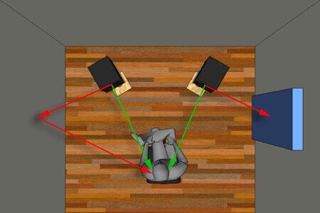
Side vs. Frontal Presentation Using Headphones vs. Loudspeakers
The Robinson-Dadson team used headphones with their participants while the Fletcher-Munson team used loudspeakers in front of the participants. There are two key differences here:
- Side versus frontal presentation of sound
- The distance of the human ear from the sound source
Headphones offer a purely side presentation of sound from a very close distance from the sound source, while loudspeakers are at a much greater distance from a more realistic angle when considering reflections in a room and in nature.
The differences in the bass measurements were attempted to be explained away by the use of headphones but the ISO report says the team used 'compensated headphones.' To this day, we aren't sure what that even means, so again it's another inconclusive excuse.
Headphones can also offer a very flat frequency response without needing acoustic treatment in the environment like loudspeakers will. This means they dodge all of the issues of constructive and deconstructive interference due to the box-shaped room.
They also avoid issues related to the shape of the ear and head and how these influence certain frequencies based on the angle at which the sound comes towards the head.
At the end of the day, no matter which method a research team uses, the other way of listening still exists and is in widespread use by listeners every day.
Perhaps the best approach would be to maintain two sets of standards, one for studio headphones and one for studio monitors, while providing an averaged summation of the two to professionals.
The Implications of the Fletcher Munson Curve
In the most simple manner of reducing all of this down to a bite-sized explanation:
If a mix is left unchanged with its tonal balance left alone, it will sound different at lower volumes and at higher volumes. At the lowest volumes, the bass and upper frequency ranges will be much quieter than the mid-range. At high volumes, bass will be more present, high frequencies can become too forward, and the mid-range will more or less remain the same with slight variance.
So how do we deal with this problem as a mastering or mixing engineer? How do we achieve a pleasing balance of frequencies for the listener no matter what volume they choose to enjoy our music or movies at?
Newcomers to the field of mixing will become extremely frustrated as they check their mixes at varying volumes, boosting and cutting and doing and un-doing the same changes over and over again, not understanding the impact of the findings in the original loudness curves.
It makes sense to say "Well, we should just mix at loud volumes, since that's when our listener's are paying the most attention anyways. If they want background noise they turn the music down anyways."
It does make sense, accept you'll end up with ear fatigue and not be able to make rational decisions during a lengthy mix session. What we need to do is mix at an average, comfortable volume for the bulk of the progress, preferably in the range of 80 to 85 dB SPL.
You need a calibrated mixing level that you always return to and come to know better than any other volume. After this, we should use our studio monitors and studio subwoofer to make adjustments at a higher volume.
This is when we'll make slight adjustments to faders, within the range of 2 dB to 5 dB and nothing more drastic. This is when we should listen critically and make some adjustments on our equalizers.
Don't keep the volume high for long. Reduce the gain and check again at an average volume and make sure it still sounds great there.

Finally, we should drop the volume to a lower amount and reference our mix on our mixing headphones. We should expect the bass and upper frequencies to be slightly more quiet than they were, relatively, but they should still sound great.
If you choose to make adjustments here, make them even slighter than you did at high volumes, because what you do here will be multiplied by two or three as you boost the volume back up.
Don't try to compensate for what consumers do. They already have their own solutions. For instance, we buy subwoofers so we can still hear the bass on our favorite songs and movies at normal volumes.
Our stereos have bass boost buttons to help compensate at low volumes. If you try to compensate first, then there will be double compensation and too much bass!
Your goal is always to produce the best result in the flattest frequency response environment possible. This minimizes all potential problems as much as possible once the audio is distributed to the masses.
You may need to repeat the mixing procedure above two or three times with tinier and tinier changes until you reach a middle ground where the mix sounds fantastic at an average-to-high volume and still sounds very good a very high volume and a low volume.
Don't drive yourself nuts though. No mixer or mastering engineer can overcome the nature of how humans perceive hearing at different volumes.
Your goal is to minimize the difference as much as possible by achieving a pleasing mix at all volumes. This mix might sound slightly different at varying volumes, but it is pleasing nonetheless.
If you enjoyed this discussion, you'll absolutely love learning about the RIAA Curve, a similar equalization curve, this time not related to our ears but to turntables and vinyl records. There's a pre-emphasis curve applied to the record which is reversed on playback to cancel each other out but reduce noise.
The Fletcher Munson Curve Conclusion
Who would have thought that we'd need to take our research to a meta-level. It's hard enough to study and develop speakers and microphones in a way that don't effect the frequency response of the sounds being produced or recorded by them.
But we also need to take into account the way our own ears and brain perceive sound across the frequency spectrum.
Thankfully, we have equal-loudness contours to help us understand the changes we need to make in our manufacturing processes and in our mixing and mastering methodologies. We give our thanks by remembering and honoring the original Fletcher Munson Curve.
Jared H.
 Jared has surpassed his 20th year in the music industry. He acts as owner, editor, lead author, and web designer of LedgerNote, as well as co-author on all articles. He has released 4 independent albums and merchandise to global sales. He has also mixed, mastered, & recorded for countless independent artists. Learn more about Jared & The LN Team here.